High Voltage and X-Ray Experiments
Text and Graphics Copyright © 2005 − 2008 Henning Umland
The following descriptions are given for the purpose of information only. I do not encourage ANYBODY to conduct experiments like those shown below, and I do not assume liability for any damage resulting from such experiments. People working with high voltage and X-rays should have a solid background in physics and electronics and should know what they are doing. The high voltage sources described here are much more powerful than generators of static electricity like, e. g., influence machines, Van de Graaff generators, etc. High voltage can kill instantly, X-rays in the long run (radiation sickness, cancer) if not handled properly.
Building a 160 kV Power Supply
Building a really powerful multiplier has been one of my most ambitious projects so far. Since the output power had to be in the kilowatt range, a full-wave multiplier was the best choice (a three-phase circuit would have been even better, but I didn't have enough components for this variant). With the available 40 kV capacitors, 160 kV output voltage could only be obtained with four doubler stages. The construction of the machine was something like an evolutionary process involving a number of experimental modifications and improvements as new ideas emerged and additional components became available. The design steps are described in chronological order.
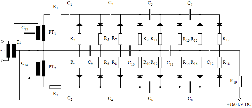
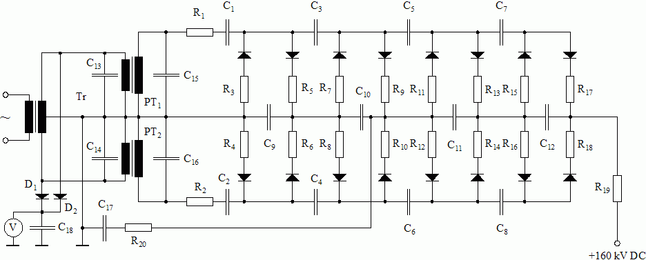
The following diagram shows the initial version of the circuit. Each HV rectifier is protected by a 2 kΩ damping resistor. Additionally, the output is protected by an array of three big 200 kΩ wire resistors (rated 500 W each). This is necessary because the capacitors store a total energy of more than 400 J at full voltage, and an accidental spark at the output would probably destroy many of the precious components if the discharge current was not limited to a tolerable value, approx. 270 mA in this case. Later, I added a fourth resistor, limiting the current to 200 mA.
|
160 kV Full-Wave Multiplier Circuit
C1...C2 = 100 nF / 20 kV, C3...C4 = 88 nF / 40 kV, C5...C6 = 66 nF / 40 kV, C7...C12 = 44 nF / 40 kV, C13...C14 = 5 μF / 400 VAC, R1...R2 = 2 k / 10 W, R3...R18 = 5.6 k / 10 W, R19 = 600 k (3 × 200 k)
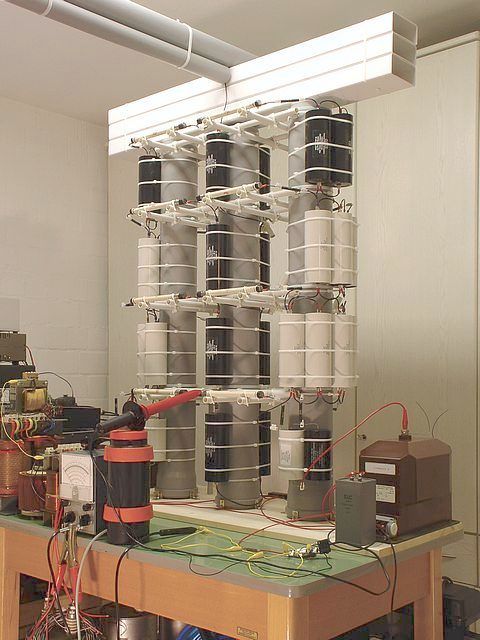
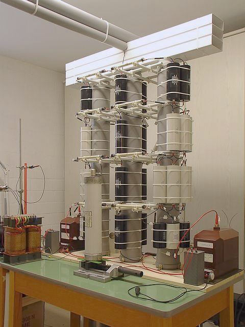
The photo shows the mechanical design of the multiplier. Simply extending the 120 kV multiplier was not possible because of limited headroom. Therefore, I had to disassemble the old machine and develop a more compact design from scratch. Due to the smaller dimensions per stage, avoiding internal arcing became a major design job. Potential difference and distance between adjacent components had to be observed very carefully. Apart from the wiring, the machine contains no metal parts (apart from a few screws and nuts at the wooden bottom plate). The mechanical structure consists of three vertical columns and a number of traverses (all polypropylene tubes and profiles) and is held together by plastic cable binders and hotmelt adhesive. The electronic components, too, are fastened with cable binders. The grey plastic tube in the upper left corner of the photo houses the big 200 kΩ resistors (each one being 33 cm long). The HV terminal is just outside the picture. The machine is ready for the first test run. On the table is a vacuum tube voltmeter. In combination with a 40 kV high-voltage probe, it measures the voltage at the first doubler stage which is one quarter of the total no-load voltage.
 |
160 kV Power Plant
The test run is spectacular. As expected, the corona discharges are even worse than with the old 120 kV multiplier.
The machine sounds like a swarm of angry bees, and a pungent ozone smell spreads instantly after turning the power
on. There are so many ions in the air that every metallic object in the room which is not grounded gets charged up.
The electrical charge in the air causes an unpleasant, itching sensation on my face. After some time, I notice that
a cupboard in the room which used to be white looks grey and shabby now. It is covered with a thin layer of
dust, forming strange patterns in some places. The dust is almost sticky and so difficult to remove that I finally
have to rub it off with alcohol because nothing else seems to work. The explanation is that dust particles in the
air capture ions and are afterwards deposited on near surfaces where they show a strong adhesion due to their electric charge. This is how electrostatic dust filters work.
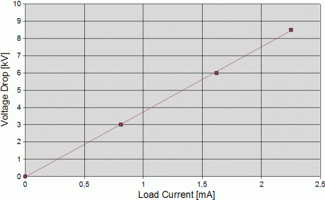
Voltage drop:
Studying the behavior of the circuit under load is the next thing to do. The diagram demonstrates that the voltage drop is a linear function of the load current. The output impedance (including the damping resistors) is 3.75 MΩ. This is not bad. When, for example, operating an X-ray tube at 100 kV anode voltage and 4 mA anode current (400 W power dissipation), the no-load voltage would have to be set at 115 kV.
 |
1st Improvement:
The circuit produces voltage spikes across the HV coils of the potential transformers exceeding the calculated peak voltage of the sine wave considerably and often triggering the safety spark gaps I installed. These transient voltages are caused by the delayed switching of the HV diodes. The KYY 29/155 is an old model with a relatively long
reverse recovery time (~1000 ns). To reduce the additional stress acting on the insulation of the HV coil, I install the capacitors C15 and C16 (1 nF, 40 kV each) which act as low-pass filters and absorb high-frequency components of the output voltage.
I further increase the capacity of C1 and C2 to 150 nF each and add the filter capacitor C17 (20 nF / 67 kV) and the damping resistor R20 (2 kΩ, 10 W) in order to decrease the output impedance of the multiplier as much as possible. C17 is rated 67 kV DC but according to the data sheet, it tolerates 130% of the rated value.
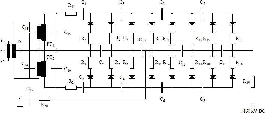 |
Upgraded Multiplier Circuit
The output impedance is approx. 3.50 MΩ now. The improvement is not really sensational but I stay with the modified version since C17 acts as a capacitive load and will certainly decrease the ripple voltage occuring under load.
2nd Improvement:
Since measuring the output voltage with the HV probe and VTVM is a little awkword, I add a simple voltage
monitoring device consisting of the diodes D1 and D2 (1N4007), the filter capacitor
C18 (20 μF), and a voltmeter. The voltage at C18 is approximately a linear function of the
no-load voltage at the HV terminal (approx. 1/800) which makes it easy to calibrate the voltmeter.
Addendum: After the 1N4007 diodes failed repeatedly when turning the equipment on (surge current), I installed a 20 Ω damping resistor in series with each diode (not shown in the circuit diagram).
 |
Multiplier Circuit with Voltmeter
This photo shows the improved version of the multiplier. The transformer on the left side is rated 3 kW and produces 2 × 150 V AC for the potential transformers which run in push-pull mode.
 |
Improved Version of 160 kV Power Plant
3rd Improvement (Final Version):
Below is the circuit diagram of the final version of the multiplier. The 11 kV HV transformers (PT1 and PT2) have been replaced with 20 kV types to avoid core saturation at full voltage (the smaller transformers got very noisy and drew a very high magnetizing current when raising the DC output voltage to more than 130 kV). TR1 is a 5 kW Variac (260V / 20A). TR2 is the 3 kW power transformer used before, this time with both 150 V secondary coils in parallel connection (shown as one coil in the diagram). TR3 is the center-tapped 230 V primary coil of a 500 W power transformer acting as a balancing choke.
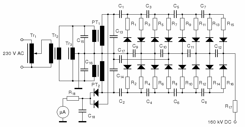 |
Final Version of Multiplier
The old 0.1 A diodes (KYY 29/155) have been replaced with 0.2 A types to improve the durability of the circuit. The new diodes are much faster (150 ns reverse recovery time) than the old ones and therefore do not produce significant voltage spikes across the transformer coils. Several capacitors have been added to the "charging stacks" (C1 thru C8) of the circuit to reduce the output impedance. The total energy stored by the capacitors is approx. 750 J now.
The circuit contains a permanent HV probe now (replacing the low-voltage probe), consisting of two HV diodes, a 3 nF load capacitor, a 1.25 GΩ resistor, and a 25 μA current meter. Instead of the peak voltage at the primary coils, the new probe measures the peak voltage at the secondary coils of the HV transformers. This is more accurate than deriving the output voltage from the primary voltage. With the 1.25 GΩ resistor, a current of 10 μA is equivalent to a peak voltage of 12.5 kV and to an output voltage (no load) of 100 kV (8×12.5 kV). The probe does not display the correct output voltage under load. This has to be calculated by subtracting the voltage drop (output impedance times load current) from the no-load voltage. Unfortunately, I presently do not have enough HV resistors to build a 160 kV probe.
Here is the updated list of
components:
| All diodes | : | 2CLG80KV/0.2A (PIV = 80 kV) |
| R1 ... R16 | : | 2 kΩ / 10 W |
| R17 | : | 800 kΩ (4 × 200 kΩ / 500 W) |
| R18 | : | 1.25 GΩ (2×500 MΩ / 20 kV + 200 MΩ / 20 kV + 50 MΩ / 10 kV) |
| C1 , C2 | : | 0.2 μF (2 × 0.1 μF / 20 kV DC) |
| C3 , C4 | : | 132 nF (6 × 22 nF / 40 kV DC) |
| C5 , C6 | : | 88 nF (4 × 22 nF / 40 kV DC) |
| C7 , C8 | : | 44 nF (2 × 22 nF / 40 kV DC) |
| C9 | : | 88 nF (4 × 22 nF / 40 kV DC) |
| C10 | : | 44 nF (2 × 22 nF / 40 kV DC) |
| C11 , C12 | : | 66 nF (3 × 22 nF / 40 kV DC) |
| C13 , C14 | : | 1 nF / 40 kV DC / 80 kV peak |
| C15 , C16 | : | 40 μF / 350 V AC |
| C17 | : | 20 nF / 67 kV DC / 87 kV peak |
| C18 | : | 3 nF / 30 kV DC |
To achieve the best efficiency, i. e., the lowest output impedance which can be achieved with a given number of capacitors, I applied the following rules this time:
C5 = 2 × C7
C3 = 3 × C7
C1 = 4 × C7
And, accordingly:
C6 = 2 × C8
C4 = 3 × C8
C2 = 4 × C8
This configuration matches the AC current distribution in the circuit better than the old design. The distribution of capacitances is more critical than I first thought. To my surprise, I observed, for example, that increasing C7 and C8 from 44 nF to 66 nF each without changing the other capacitors was not only inefficient but actually had a detrimental effect (slightly increasing the output impedance). The capacitance of C1 and C2 (0.2 μF each) is slightly higher than calculated (176 nF). This is mainly because I happended to have a number of rugged 0.1 μF / 20 kV capacitors in stock. At this position, a higher capacitance decreases the output impedance slightly.
To understand how the circuit works, one can imagine it as a series stack of four full-wave rectifier bridges
in which the (+) terminal of each bridge is connected with the (−) terminal of the following bridge. The
average DC current flowing through each HV diode is exactly half the load current of the multiplier. The AC
input current is fed into each bridge through a pair of capacitors which conduct AC current but block any
DC current resulting from the potential diffence between adjacent stages. The circuit diagram shows that
C7 and C8 feed one bridge (the one connected to the HV terminal), C5
and C6 feed two bridges, C3 and C4 three bridges, and so on. Since
each rectifier bridge draws the same AC current, the AC current flowing through a chosen pair of feeder
capacitors is proportional to the number of bridges it has to feed. To achieve the same AC voltage drop, each
capacitance has to be proportional to the respective AC current. I chose heavy-duty pulse capacitors for
C1 and C2 since these capacitors, feeding all rectifier bridges, have to bear the
highest AC current in the circuit.
The load capacitors of the rectifier bridges (C9 thru C12 and C17)
act almost exclusively as low-pass filters and have little influence on the output impedance. Their capacitance
is not critical and can be chosen according to the tolerable ripple voltage at a given load current. Since
these capacitors bear the same dynamic load, their capacitances should be equal. I deviated from this layout
slighly by adding C17 and increasing C9 to 88 nF because I sometimes use the
lower stages of the multiplier as low-voltage taps for applications requiring higher current.
I use the following simple method to measure the output impedance of a multiplier. First, the open-circuit voltage, U0, measured with a HV probe and a VTVM, is adjusted to 40 kV (the maximum voltage my HV probe can handle). Then, the power is turned off, the circuit discharged, the HV probe and VTVM replaced with a current meter, and the power turned on again. Now, the current meter measures the corresponding short-circuit current, IS. The output impedance, Z, is
Z = U0 / IS
With the new configuration, the output impedance of the multiplier is approx. 2.5 MΩ. Under load, the voltage drop across the damping resistors (800 kΩ) is about one third of the total voltage drop, i. e., the output impedance of the multiplier itself is about 1.7 MΩ. The above method for measuring the output impedance would not work without the damping resistors because the U-I relationship of a multiplier is approximately linear only under moderate load. The curve flattens out when the output voltage of the multiplier becomes smaller than about one third of the no-load voltage.
The following calculation shows how powerful the multiplier is. At 160 kV no-load voltage, the short-circuit current is 64 mA. The resulting voltage drop across the four damping resistors (4×200 kΩ) is 51.2 kV. Thus, the total power dissipated by the resistor array is 3277 W!
Under practical conditions, it is possible to draw a current of 10 mA at 135 kV output voltage (P = 1350 W) for some time when setting the no-load voltage at 160 kV. The duty cycle is only limited by the power dissipated in the damping resistors (200 W per resistor).
Here is a photo of the final version:
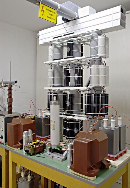 |
Final Version of Multiplier
Low-voltage side:
Here is a photo of the low-voltage part of the equipment. On the left side is a remote-controlled soft-start circuit with 2 relays and a big 22 Ω wire resistor limiting the surge current to approx. 15 A when starting the equipment. The grey box in the middle houses the 5 kW variac (260 V / 20 A) feeding the 3 kW power transformer (right).
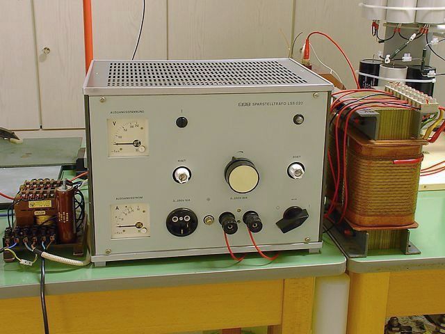 |
Low-Voltage Equipment
Discharge experiments:
Out of curiosity, I build an improvised spark gap using two cylindrical steel rods (see next photo). The left rod is
connected to the HV terminal, the right one is fastened to a grounded lab stand. I set the gap at 30 cm (12").
When I slowly increase the voltage, visible corona discharges occur at about 100 kV, getting more intense as the
voltage increases further. At full power (160 kV), sparking occurs almost immediately. After ignition, the arc keeps
burning until I turn the power off to keep the rectifiers from overheating. Later, I find that the rectifiers are on
the safe side because the average current flowing through the arc is limited to approx. 60 mA by the voltage drop under load. However, such a load current should not be maintained permanently because of the AC current flowing through the capacitors, increasing the stress acting on the dielectric.
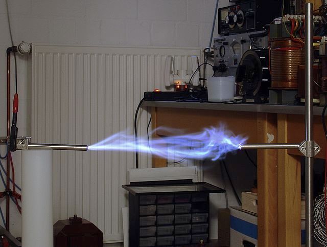 |
30 cm (12") Arc Discharge at 160 kV DC
30 cm is about the maximum spark length I observe at full voltage. When the gap between the electrodes is wider, there are only strong corona discharges. Since nobody wants to get hit by such a spark, a safety distance of at least 1.5 m (6 ft) is highly recommended. I use a remote-controlled relay to turn the power on and off, and I make it a habit to discharge the capacitors after each experiment by shorting the HV terminal to ground.
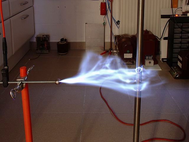
The next picture shows a continuous arc burning between two spherical (d = 15 mm) steel electrodes. As expected, the maximum arc length is smaller than before, 28 cm in this case.
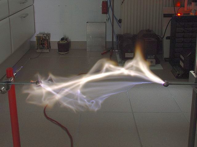 |
28 cm Discharge between Spherical Electrodes (d = 15 mm)
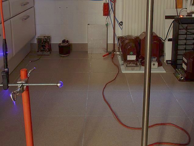
Here is a photo taken from a greater distance:
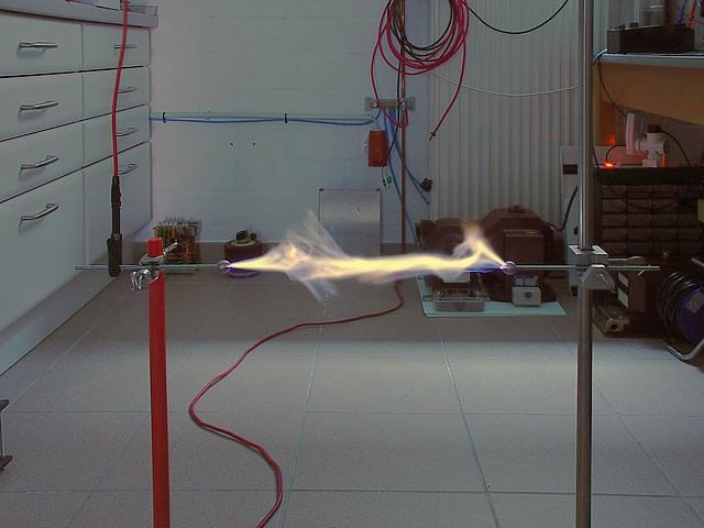 |
Another 28 cm Arc Discharge
For the next experiment, I replace the negative electrode with a vertical steel rod (20 mm diameter). Now, the maximum discharge length is reduced to 18 cm.
 |
18 cm Arc Discharge
For the next photo, the spark gap was set at 19 cm, just above the maximum spark length. The time exposure shows corona discharges on the anode side, even on the surface of the steel sphere.
 |
Corona Discharge